User guide
Introduction
We start off by giving some mathematical background, or rather by defining the needed language.
Weakly separated Collections
For any integer $n \geq 1$ we use the notation $[n]:=$ { $1, 2, \ldots, n$ } and denote by $\text{Pot}(k,n)$ the set of $k$-subsets of $[n]$.
Definition (weak separation)
Let $I, J$ be $k$-subsets of $[n]$, then we call $I$ and $J$ $\textbf{weakly separated}$ if we cannot find elements $a, c \in I \setminus J$ and $b, d \in J \setminus I$ such that $(a, b, c, d)$ is strictly cyclically ordered. In this case we write $I \parallel J$.
Intuitively two $k$-subsets are weakly separated if after can arranging $I \setminus J$ and $J \setminus I$ clockwise on a circle, they can be separated by a line.
Definition (weakly separated collection)
A subset $\mathcal{C} \subseteq \text{Pot}(k,n)$ is called a $\textbf{weakly separated collection}$ (abbreviated by WSC) if its elements are pairwise weakly separated. We often referr to elements of a WSC as labels.
Definition (mutation)
If $\mathcal{C}$ is a WSC that includes sets of the form $Iab, Ibc, Icd, Iad$ and $Iac$, where $(a,b,c,d)$ is strictly cyclically ordered. Then $\mathcal{C'} = (\mathcal{C} \setminus \{Iac\}) \cup \{Ibd\}$ is also a weakly separated collection, and we call the exchange of $Iac$ by $Ibd$ a $\textbf{mutation}$.
Plabic Tilings
Definition (plabic tiling)
Any WSC can be given the structure of an abstract $2$-dimensional cell complex, which in turn may be embedded into the plane. This construction will be called an (abstract) $\textbf{plabic tiling}$, and we referr to Weak Separation and Plabic Graphs.
Intuitively a plabic tiling is a tiling of a convex $n$-gon into convex polygons, colored either black or white, and with vertices labelled by the elements of the underlying WSC. Plabic tilings are in bijective correspondance with WSC's that are maximal with respect to inclusion.
Plabic Graphs
Definition (plabic graph)
A $\textbf{plabic graph}$ is a finite simple connected plane graph $G$ whose interior is bounded by a vertex disjoint cycle containing $n$ $\textbf{boundary vertices}$ $b_1, \ldots, b_n$. Here the labelling is chosen in clockwise order.
We only consider $\textbf{reduced}$ plabic graphs which can be also seen to be in one to one correspondance to WSC's that are maximal with respect to inclusion. For more details we referr to Total positivity, Grassmannians, and networks.
Creating WSC's
In this package we use vecors in place of sets, although WSC's are by definition sets of $k$-sets. We always assume such vectors to be increasingly ordered and not contain double elements. None of the below methods check these properties and unforseen behavior may arise if they are not fulfilled.
The data type for WSC's or rather (abstract) plabic tilings is given by WSCollection.
WeaklySeparatedCollections.WSCollection — TypeWSCollectionAn abstract 2-dimensional cell complex living inside the matriod of k-sets in {1, ..., n}. Its vertices are labelled by elements of labels while quiver encodes adjacencies between the vertices. The 2-cells are colored black or white and contained in blackCliques and whiteCliques.
Attributes
k::Intn::Intlabels::Vector{Vector{T}}quiver::SimpleDiGraph{T}whiteCliques::Dict{Vector{T}, Vector{T}}blackCliques::Dict{Vector{T}, Vector{T}}
Constructors
WSCollection(k::Int, n::Int, labels::Vector{Vector{T}},
            computeCliques::Bool = true, frozenFirst::Bool = true)

WSCollection(k::Int, n::Int, labels::Vector{Vector{T}}, quiver::SimpleDiGraph{T},
            computeCliques::Bool = true, frozenFirst::Bool = true)

WSCollection(C::WSCollection; computeCliques::Bool = true)Constructors
There are three different constructors to create a WSC:
WeaklySeparatedCollections.WSCollection — MethodWSCollection(k::Int, n::Int, labels::Vector{Vector{Int}}, computeCliques::Bool = true)Constructor of WSCollection. Adjacencies between its vertices as well as 2-cells are computed using only a set of vertex labels.
If computeCliques is set to false, the 2-cells will be left empty.
WeaklySeparatedCollections.WSCollection — MethodWSCollection(k::Int, n::Int, labels::Vector{Vector{Int}}, quiver::SimpleDiGraph{Int},
computeCliques::Bool = true)Constructor of WSCollection. The 2-cells are computed from vertex labels as well as the their adjacencies encoded in quiver. Faster than just using labels most of the time.
If computeCliques is false the black and white 2-cells are are left empty instead.
WeaklySeparatedCollections.WSCollection — MethodWSCollection(C::WSCollection; computeCliques::Bool = true)Constructor of WSCollection. Computes 2-cells of C if the are empty, othererwise returns a deepcopy of C.
If computeCliques is false the black and white 2-cells are left empty instead.
Thus to construct a WSC we only need to know its labels.
Examples:
If we are not sure about the weak spearation of a given set of labels, we can easily test it.
labels = [[1, 5, 6], [1, 2, 6], [1, 2, 3], [2, 3, 4], [3, 4, 5],
          [4, 5, 6], [2, 5, 6], [2, 3, 6], [3, 5, 6], [3, 4, 6] ]
is_weakly_separated(labels) # checks for pairwise weak separationtrueC = WSCollection(3, 6, labels)WSCollection{Int64} of type (3, 6) with 10 labelsHowever, if the underlying quiver is already known it can be passed to the constructor to speed up computations.
Q = C.quiver
WSCollection(3, 6, labels, Q)
WSCollection{Int64} of type (3, 6) with 10 labelsThe last constructor is useful, if we already have a WSC but want to omit the 2-cells or if the 2-cells of our WSC are empty and we want to compute them.
D = WSCollection(C, computeCliques = false)
cliques_empty(D) # checks if the cliques (i.e. the 2-cells) are emptytrueD = WSCollection(D)
D.whiteCliquesDict{Vector{Int64}, Vector{Int64}} with 5 entries:
[2, 3] => [3, 4, 8]
[5, 6] => [1, 7, 9, 6]
[2, 6] => [2, 8, 7]
[3, 4] => [4, 5, 10]
[3, 6] => [8, 10, 9]Extending to maximal collections
Sometimes we only want some maximal WSC containing one or more disired labels. To obtain such WSC's we simple add labels to our desired as long as possible.
WeaklySeparatedCollections.extend_weakly_separated! — Functionextend_weakly_separated!(k::Int, n::Int, labels::Vector{Vector{T}})Extend labels to contain the labels of a maximal weakly separated collection.
extend_weakly_separated!(k::Int, n::Int, labels1::Vector{Vector{T}},
                                         labels2::Vector{Vector{T}})
Extend labels1 to contain the labels of a maximal weakly separated collection. Use elements of labels2 if possible.
extend_weakly_separated!(labels::Vector{Vector{Int}}, C::WSCollection)Extend labels to contain the labels of a maximal weakly separated collection. Use labels of C if possible.
WeaklySeparatedCollections.extend_to_collection — Functionextend_to_collection(k::Int, n::Int, labels::Vector{Vector{Int}})Return a maximal weakly separated collection containing all elements of labels.
extend_to_collection(k::Int, n::Int, labels1::Vector{Vector{Int}},
                                     labels2::Vector{Vector{Int}})
Return a maximal weakly separated collection containing all elements of labels1. Use elements of labels2 if possible.
extend_to_collection(labels::Vector{Vector{Int}}, C::WSCollection)Return a maximal weakly separated collection containing all elements of labels. Use labels of collection if possible.
Examples:
We may extend using brute force:
label = [1, 3, 4]
extend_weakly_separated!(3, 6, [label])
10-element Vector{Vector{Int64}}:
[1, 5, 6]
[1, 2, 6]
[1, 2, 3]
[2, 3, 4]
[3, 4, 5]
[4, 5, 6]
[1, 3, 4]
[1, 2, 4]
[1, 2, 5]
[1, 4, 5]Or if we want to prefer labels from a known weakly separated set (and then fill up by brute force):
label = [1, 3, 4]
preferred_labels = [[1, 5, 6], [1, 2, 6], [1, 2, 3], [2, 3, 4], [3, 4, 5],
                    [4, 5, 6], [2, 5, 6], [2, 3, 6], [3, 5, 6], [3, 4, 6]]
extend_weakly_separated!(3, 6, [label], preferred_labels)
10-element Vector{Vector{Int64}}:
[1, 5, 6]
[1, 2, 6]
[1, 2, 3]
[2, 3, 4]
[3, 4, 5]
[4, 5, 6]
[1, 3, 4]
[3, 5, 6]
[3, 4, 6]
[1, 3, 6]We could have just as well passed a WSC instead of preferred_labels above. Note that so far we only constructed arrays of labels. To obtain a WSC containing these labels we use extend_to_collection.
label = [1, 3, 4]
extend_to_collection(3, 6, [label], preferred_labels)
WSCollection{Int64} of type (3, 6) with 10 labelsPredefined collections
We provide shortcuts for the construction of some well known WSC's:
WeaklySeparatedCollections.checkboard_collection — Functioncheckboard_collection(k::Int, n::Int, T::Type = Int)Return the weakly separated collection corresponding to the checkboard graph.
WeaklySeparatedCollections.rectangle_collection — Functionrectangle_collection(k::Int, n::Int, T::Type = Int)Return the weakly separated collection corresponding to the rectangle graph.
WeaklySeparatedCollections.dual_checkboard_collection — Functiondual_checkboard_collection(k::Int, n::Int, T::Type = Int)Return the weakly separated collection corresponding to the dual-checkboard graph.
WeaklySeparatedCollections.dual_rectangle_collection — Functiondual_rectangle_collection(k::Int, n::Int, T::Type = Int)Return the weakly separated collection corresponding to the dual-rectangle graph.
Examples:
rectangle_collection(3, 6)WSCollection{Int64} of type (3, 6) with 10 labelsIf we only want the underlying labels we may instead use rectangle_labels(k::Int, n::Int) (similar for the other predefined collections).
rectangle_labels(3, 6)10-element Vector{Vector{Int64}}:
[1, 5, 6]
[1, 2, 6]
[1, 2, 3]
[2, 3, 4]
[3, 4, 5]
[4, 5, 6]
[2, 5, 6]
[2, 3, 6]
[3, 5, 6]
[3, 4, 6]The labels of the rectangle collection can be arranged on a grid in a natural way. Specific labels in this grid are returned by rectangle_label(k::Int, n::Int, i::Int, j::Int) where $i = 0, ..., n-k$ and $j = 0, ..., k$ (similar for the other collections, where for the dual ones $i = 0, ..., k$ and $j = 0, ..., n-k$ ).
rectangle_label(3, 6, 1, 2)3-element Vector{Int64}:
2
3
6Basic functionality
Armed with this plethora of examples, we are ready to discuss the basic functionalities of WSC's.
WSC's behave in many ways as their underlying arrays of labels would. In particular labels may be accessed directly.
rec = rectangle_collection(3, 6)
rec[3]
3-element Vector{Int64}:
1
2
3rec[[1, 7]]2-element Vector{Vector{Int64}}:
[1, 5, 6]
[2, 5, 6]For convenience we also extend the following functions:
Base.in — Functionin(label::Vector{Int}, C::WSCollection)Return true if label is occurs as label of C.
Base.length — Functionlength(C::WSCollection)Return the length of C.labels.
Base.intersect — Functionintersect(C1::WSCollection, C2::WSCollection)Return the common labels of C1 and C2.
Base.setdiff — Functionsetdiff(C1::WSCollection, C2::WSCollection)Return the labels of C1 minus the labels of C2.
Base.union — Functionsetdiff(C1::WSCollection, C2::WSCollection)Return the union of labels in C1 and C2.
Examples:
rec = rectangle_collection(3, 6)
check = checkboard_collection(3, 6)

check[10] in recfalselength(check)10intersect(rec, check) # similar for union and setdiff6-element Vector{Vector{Int64}}:
[1, 5, 6]
[1, 2, 6]
[1, 2, 3]
[2, 3, 4]
[3, 4, 5]
[4, 5, 6]Mutation
WSC's usually contain frozen elements that never change. On the other hand some elements may be modified via mutation and are called mutable. To figure out which elements of a WSC are frozen or mutable use the functions is_frozen or is_mutable.
WeaklySeparatedCollections.is_frozen — Functionis_frozen(C::WSCollection, i::Int)Return true if the vertex i of C is frozen.
is_frozen(seed::Seed, i::Int)Return true if the i-th clustervariable of seed is frozen.
WeaklySeparatedCollections.is_mutable — Functionis_mutable(C::WSCollection, i::Int)Return true if the vertex i of C is mutable.
rec = rectangle_collection(3, 6)
is_frozen(rec, 4)trueis_mutable(rec, 7)trueis_mutable(rec, 8)falseThe frozen labels contained in any (maximal) WSC can be obtained via
WeaklySeparatedCollections.frozen_label — Functionfrozen_label(k::Int, n::Int, i::Int)Return the i-th frozen label.
WeaklySeparatedCollections.frozen_labels — Functionfrozen_labels(k::Int, n::Int)Return the frozen labels as a vector.
The indices of the mutable labels on a WSC can be obtained by using
WeaklySeparatedCollections.get_mutables — Functionget_mutables(C::WSCollection)Return all mutable vertices of C.
Finally, to mutate a WSC in the direction of a mutable label, the functions mutateand mutate! are available.
WeaklySeparatedCollections.mutate! — Functionmutate!(C::WSCollection, i::Int, mutateCliques::Bool = true)Mutate the C in direction i if i is a mutable vertex of C.
If mutateCliques is set to false, the 2-cells are emptied.
mutate!(C::WSCollection, label::Vector{T}, mutateCliques::Bool = true)Mutate the C by addressing a vertex with its label.
mutate!(seed::Seed, i::Int)Mutate the seed in direction i if i is the index of a mutable variable.
WeaklySeparatedCollections.mutate — Functionmutate(C::WSCollection, i::Int, mutateCliques::Bool = true)Version of mutate! that does not modify its arguments.
mutate(C::WSCollection, label::Vector{Int}, mutateCliques::Bool = true)Mutate the C by addressing a vertex with its label, without modifying arguments.
mutate(seed::Seed, i::Int)Mutate the seed in direction i if i is the index of a mutable variable.
Examples:
rec = rectangle_collection(3, 6)
get_mutables(rec)
3-element Vector{Int64}:
7
9
10mutate!(rec, 7)
println(rec, full = true)WSCollection{Int64} of type (3, 6) with 10 labels:
[1, 5, 6]
[1, 2, 6]
[1, 2, 3]
[2, 3, 4]
[3, 4, 5]
[4, 5, 6]
[1, 3, 6]
[2, 3, 6]
[3, 5, 6]
[3, 4, 6]For convenience we may also mutate by specifying a label:
mutate!(rec, [3,4,6])
println(rec, full = true)
WSCollection{Int64} of type (3, 6) with 10 labels:
[1, 5, 6]
[1, 2, 6]
[1, 2, 3]
[2, 3, 4]
[3, 4, 5]
[4, 5, 6]
[1, 3, 6]
[2, 3, 6]
[3, 5, 6]
[2, 3, 5]Other transformations
Apart from mutation, several other transformations of WSC's are available:
WeaklySeparatedCollections.rotate! — Functionrotate!(C::WSCollection, amount::Int = 1)Rotate C by amount, where a positive amount indicates a clockwise rotation.
WeaklySeparatedCollections.mirror! — Functionmirror!(C::WSCollection, shift::Int = 2)Reflect C by letting the permutation p(x) = shift - x interpreted modulo n = C.n act on the labels of C.
WeaklySeparatedCollections.complements! — Functioncomplements!(C::WSCollection)Return the collection whose labels are complementary to those of C.
WeaklySeparatedCollections.swap_colors! — Functionswap_colors!(C::WSCollection)Return the weakly separated collection whose corresponding plabic graph is obtained from the one of C by swapping the colors black and white.
This is the same as taking complements and rotating by C.k.
For each of the above methods, a variant that does not modify its argument is avaliable (just omit the ! ).
Examples:
check = checkboard_collection(3, 6)
check.labels
10-element Vector{Vector{Int64}}:
[1, 5, 6]
[1, 2, 6]
[1, 2, 3]
[2, 3, 4]
[3, 4, 5]
[4, 5, 6]
[1, 4, 5]
[1, 4, 6]
[1, 3, 4]
[1, 2, 4]check = checkboard_collection(3, 6)
rotate!(check, 1)
check.labels10-element Vector{Vector{Int64}}:
[1, 2, 6]
[1, 2, 3]
[2, 3, 4]
[3, 4, 5]
[4, 5, 6]
[1, 5, 6]
[2, 5, 6]
[1, 2, 5]
[2, 4, 5]
[2, 3, 5]mirror!(check, 1)
check.labels10-element Vector{Vector{Int64}}:
[1, 5, 6]
[4, 5, 6]
[3, 4, 5]
[2, 3, 4]
[1, 2, 3]
[1, 2, 6]
[1, 2, 5]
[2, 5, 6]
[2, 3, 5]
[2, 4, 5]Searching
In theory all WSC's of common type can be transformed into each other by mutations. In proctice however it is quite difficult to find a suitable sequence of mutations from one WSC to another. Thus we provide different searching algorithms to automate the search for such sequences.
On the conceptually easy end we have breadth and depth first search:
WeaklySeparatedCollections.BFS — FunctionBFS(root::WSCollection, target::WSCollection)Return a minimal sequence of mutations, transforming root into target. This sequence is computed by a breadth first search.
Keyword arguments:
limitSearchSpace::Bool = true
If limitSearchSpace is set to true then labels already contained in target will never be mutated.
WeaklySeparatedCollections.DFS — FunctionDFS(root::WSCollection, target::WSCollection)Return a sequence of mutations, transforming root into target. This sequence is computed by a depth first search.
Keyword arguments:
limitSearchSpace::Bool = true
If limitSearchSpace is set to true then labels already contained in target will never be mutated.
Examples:
check = checkboard_collection(3, 7)
rec = rectangle_collection(3, 7)
BFS(check, rec)
8-element Vector{Int64}:
8
10
9
11
10
12
13
11DFS(check, rec)144-element Vector{Int64}:
13
12
13
12
11
13
9
13
12
11
⋮
12
11
13
12
13
8
13
12
11If the target WSC is close enough, searching is also feasable for bigger parameters.
check = checkboard_collection(7, 16)
label = [1, 2, 3, 4, 5, 6, 15]
target = extend_to_collection([label], check)
DFS(check, target, limitSearchSpace = true)
9-element Vector{Int64}:
46
39
32
25
18
19
26
33
40For more informed searching we first need suitable heuristics, i.e. lower bounds on the number of mutations needed to reach a WSC from a given one.
WeaklySeparatedCollections.number_wrong_labels — Functionnumber_wrong_labels(C::WSCollection, target::WSCollection)Return the number of labels in C that do not occur in target.
WeaklySeparatedCollections.min_label_dist — Functionmin_label_dist(C::WSCollection, target::WSCollection)Return the sum of minimum label distances, where for each label in C this distance is calculated as the minimal number of integer pairs one needs to exchange in order to obtain a label of target.
WeaklySeparatedCollections.min_label_dist_experimental — Functionmin_label_dist_experimental(C::WSCollection, target::WSCollection)Return the sum over minimal label distances of wrong labels in C.
This assumes that a minimal sequence of mutations between WSC's can be found while never mutating correct labels i.e. labels that are contained in the target WSC.
Examples:
check = checkboard_collection(10, 20)
rec = rectangle_collection(10, 20)
number_wrong_labels(check, rec)81min_label_dist(check, rec)121min_label_dist_experimental(check, rec)121The above heuristics can be used for the Astar algorithm by passing the corresponding enum.
WeaklySeparatedCollections.Astar — FunctionAstar(root::WSCollection, target::WSCollection)Return a minimal sequence of mutations, transforming root into target. This sequence is computed by a the astar algorithm.
Keyword arguments:
heuristic::String = "number_wrong_labels"limitSearchSpace::Bool = true
The available heuristic's are "number_wrong_labels", "min_label_dist" and "min_label_dist_experimental". If limitSearchSpace is set to true then labels already contained in target will never be mutated.
Examples:
check = checkboard_collection(3, 8)
rec = rectangle_collection(3, 8)
Astar(check, rec)
11-element Vector{Int64}:
9
11
10
12
13
14
11
15
16
12
15check = checkboard_collection(4, 9)
rec = rectangle_collection(4, 9)
Astar(check, rec, heuristic = "min_label_dist_experimental")20-element Vector{Int64}:
10
13
11
14
16
12
13
17
18
20
19
15
17
14
21
12
20
17
18
20Sometimes we only want to find a sequence of mutations from some WSC to any WSC containing some desired label.
WeaklySeparatedCollections.find_label — FunctionAstar(root::WSCollection, target::WSCollection)Returns a sequence of mutations, transforming root into a wsc containing label.
This sequence is computed by a the astar algorithm.
Keyword arguments:
heuristic::String = "number_wrong_labels"limitSearchSpace::Bool = true
The available heuristic's are "number_wrong_labels", "min_label_dist" and "min_label_dist_experimental". If limitSearchSpace is set to true then labels already contained in target will never be mutated.
check = checkboard_collection(4, 9)
label = [2, 3, 4, 9]
s = find_label(check, label, heuristic = "min_label_dist_experimental")
6-element Vector{Int64}:
10
14
18
13
17
21Lets test the found sequence
for i in s
    mutate!(check, i)
end

check[21] # = label
4-element Vector{Int64}:
2
3
4
9Finally to get an overview we can calculate all WSC's of a given type and connect those who arise from each other by mutation by an edge. The resulting Graph is also called the generalized associahedron.
WeaklySeparatedCollections.generalized_associahedron — Functiongeneralized_associahedron(root::WSCollection)Return all maximal weakly separated collections of same type as root together with a graph that decribes mutations between the wsc's.
generalized_associahedron(root::WSCollection)Return all maximal weakly separated collections of type k, n together with a graph that decribes mutations between the wsc's.
root = checkboard_collection(3, 7)
list, A = generalized_associahedron(root)
A
{259, 644} undirected simple Int64 graphThe obtained Graph may be plotted in 3D using external libraries such as GraphMakie:
max = length(root) - root.n
n_mutables = a -> length(get_mutables(list[a]))
min = minimum(n_mutables(a) for a in 1:nv(A))
d = max - min

# greener means more mutable faces, red means less mutable faces.
node_colors = [RGBA(1.0 - (n_mutables(a) - min)/d, (n_mutables(a) - min)/d, 0.0, 1.0)
                for a in 1:nv(A)]

graphplot(A, layout = Spring(dim = 3, seed = 1), edge_width = 0.5, node_size = 15,
            node_color = node_colors)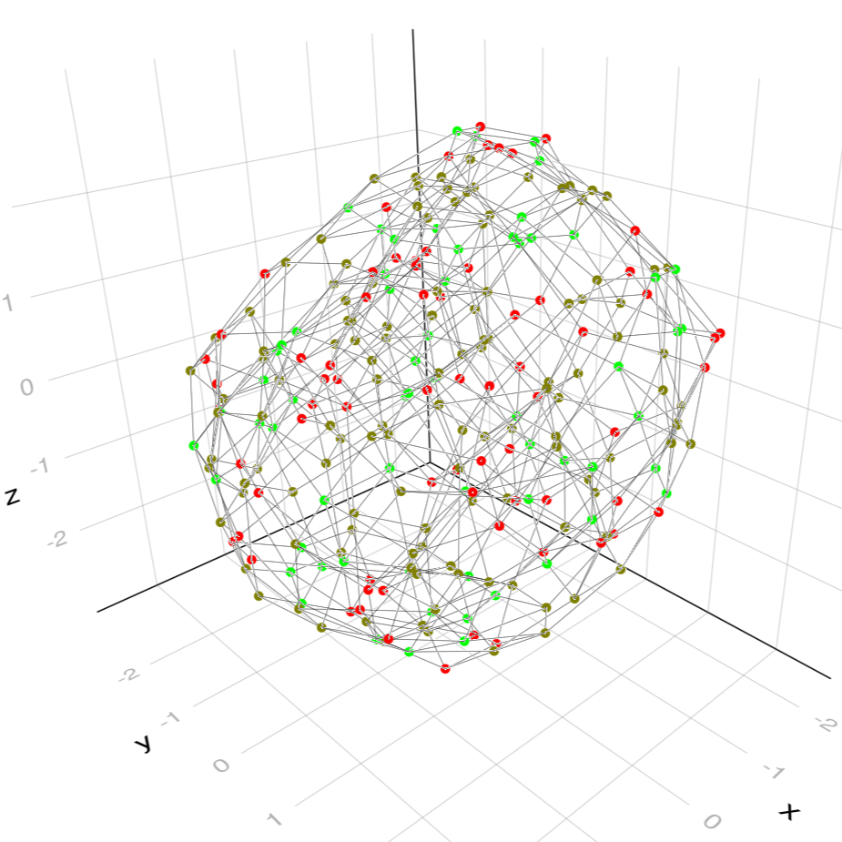
Plotting
Plotting WSC's requires Luxor to be installed and loaded as detailed here.
plotting is currently only available for maximal weakly separated collections.
In the introduction we learned about plabic tilings as well as plabic graphs as objects living in the plane which are in one to one correspondance to maximal WSC's. Thus we can plot a maximal WSC using its corresponding plabic tiling or plabic graph. The functions to accomplish this are:
WeaklySeparatedCollections.drawTiling — FunctiondrawTiling(collection::WSCollection, title::String, width::Int = 500, height::Int = 500)Draw the plabic tiling of the provided weakly separated collection and save it as an image file of specified size. Both the name as well as the resulting file type of the image are controlled via title.
Inside a Jupyter sheet drawing without saving an image is possible by omitting the title argument i.e. via drawTiling(collection::WSCollection, width::Int = 500, height::Int = 500).
Keyword Arguments
topLabel = nothingbackgroundColor::Union{String, ColorTypes.Colorant} = ""drawLabels::Bool = truehighlightMutables::Bool = truelabelDirection = "left"
toplabel controls the rotation of the drawing by drawing the specified label at the top. labelDirection controls whether the "left" (i.e. the usual ones) or "right" (complementss) labels are drawn.
WeaklySeparatedCollections.drawPLG — FunctiondrawPLG(collection::WSCollection, title::String, width::Int = 500, height::Int = 500)Draw the plabic graph of the provided weakly separated collection and save it as an image file of specified size. Both the name as well as the resulting file type of the image are controlled via title.
Inside a Jupyter sheet drawing without saving an image is possible by omitting the title argument i.e. via drawPLG(collection::WSCollection, width::Int = 500, height::Int = 500).
Keyword Arguments
topLabel = nothingdrawmode::String = "straight"backgroundColor::Union{String, ColorTypes.Colorant} = ""drawLabels::Bool = truehighlightMutables::Bool = falselabelDirection = "left"
toplabel controls the rotation of the drawing by drawing the specified label at the top. drawmode controls how edges are drawn and may be choosen as "straight", "smooth" or "polygonal". labelDirection controls whether the "left" (i.e. the usual ones) or "right" (complementss) labels are drawn.
Examples:
If working in a Jupyter sheet, WSC's may be plottet directly without saving the image in a file.
H = rectangle_collection(3, 6)
drawTiling(H) # plotts H as plabic tiling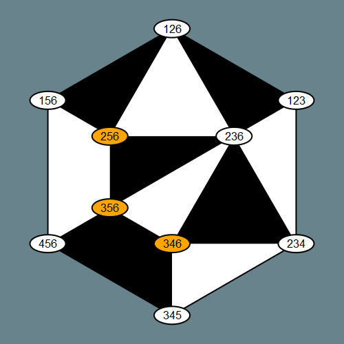
H = rectangle_collection(3, 6)
drawPLG_straight(H; drawLabels = true) # plotts H as plabic graph with straight edges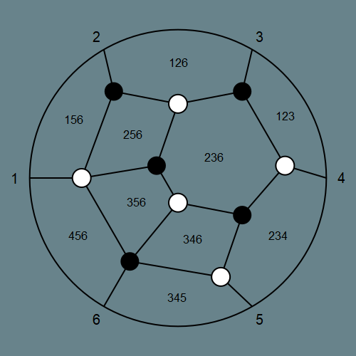
To save an image as png, svg, pdf or eps file, we just need to give it a title with the corresponding file extension.
H = checkboard_collection(3, 6)
# will save the image as title.png (by defalut without background)
drawPLG_straight(H, "title.png"; drawLabels = true)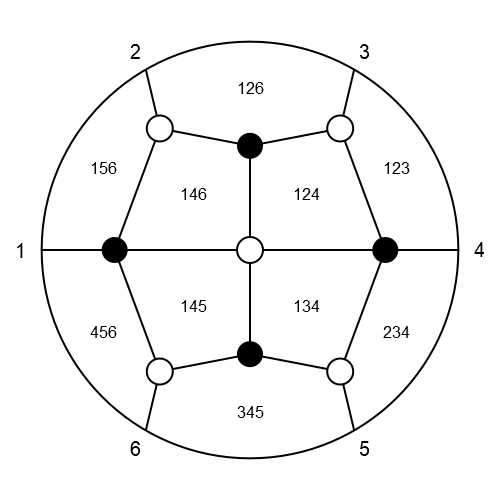
Graphical user interface
The graphical user interface requires both an installation of Luxor as well as Mousetrap. See here for details.
While plotting WSC's enables us to visualize them, the resulting images lack interactivity. This is where the built in gui application comes in handy. To start it we use
WeaklySeparatedCollections.visualizer! — Functionvisualizer!(collection::WSCollection = rectangle_collection(4, 9))Start the graphical user interface to visualize the provided collection.
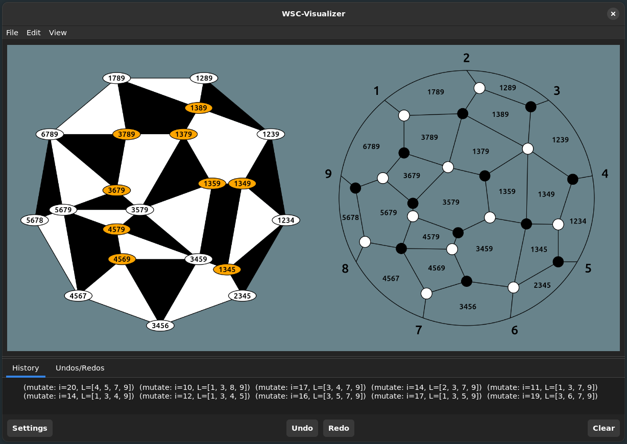
Much of the functionality discussed so far is available through this interface, for example to mutate a WSC in the direction of a label we can just click on it.
We shortly explain the content of the menubar as well as settings.
Settings
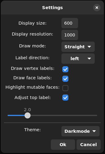
Draw modecontrols how edges of the plabic graph are drwn. The available modes areStraight,SmoothandPolygonalLabel directioncontrols whether the left (i.e. the usual ones) or right labels (complements of left labels) are drawn.Draw vertex labelscontrols if the labels in the plabic tiling should be drawn or not.Draw face labelscontrols whether the labels in the plabic graph are drawn or not.Highlight mutable facesenables the highlighting of mutable faces of the plabic graph. This only works if the drawmode is set toStraight.adjust top labelif checked then a the boundary label of the plabic graph that should be drawn at the top can be chosen through the slider below. This adjusts both the embedding of the plabic graph as well as the corresponding tiling.
File
Through the File submenu we may save or load WSC's.
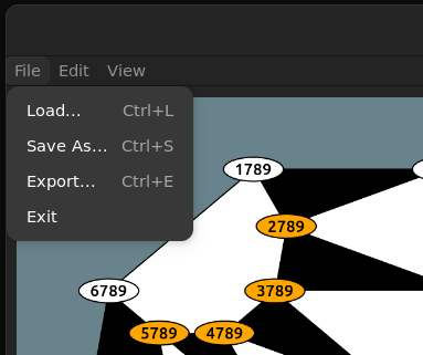
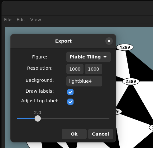
Moreover we can also easily export the images drawn in the gui as png, svg, pdf or eps file
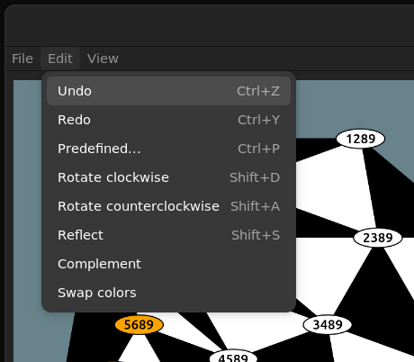
Edit
The Edit submenu contains transformations other than mutation, such as rotations and reflections as well as a quick way to load all the predefines WSC's.
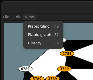
View
Finally under the view submenu all options to disable/enable parts of the gui are collected.
Oscar extension
This extension requires an installation of Oscar Oscar (see also the Oscar website).
The action of the dihedral group
There is a natural action of the dihedral group on WSC's (realised as permutation group) induced by applying permutations to $k$-sets.
Most computer algebra systems, in particular Oscar, preferr rigth actions over left actions. Thus a permutation $\pi \in S_n$ is applied to $x \in [n]$ from the right. We define $x^\pi := \pi(x)$. As a consequence we need to consider Permutation groups with the opposite product $\pi * \tau := \tau \circ \pi$, where the right hand side is the usual composition of functions. This ensures $x^{\pi * \tau} = (x^\pi)^\tau$.
Base.:^ — Function^(collection::WSCollection, p::PermGroupElem)Let p act on collection via the natural right action.
We extend several Oscar functions to simplify their usage with WSC's. We urge the reader to consult the Oscar documentaion, specifically the sections Permutation Groups and Group Actions for more information about their usage.
Oscar.gset — Functiongset(D::PermGroup, seeds::Vector{WSCollection}; closed::Bool = false)Return the G-set of the natural action of D on the specified WSC's in seeds.
Hecke.orbit — Functionorbit(D::PermGroup, collection::WSCollection)Return the orbit of collection under the natural action of D.
orbit(collection::WSCollection)Return the orbit of collection under the natural action of the dihedral group.
Hecke.stabilizer — Functionstabilizer(D::PermGroup, collection::WSCollection)Return the stabilizer of collection under the natural action of D.
stabilizer(collection::WSCollection)Return the stabilizer of collection under the natural action of the dihedral group.
Examples:
s, t = cperm(collect(1:6)), perm([1, 6, 5, 4, 3, 2])
check = checkboard_collection(3, 6)

println(check^t, full = true)
WSCollection{Int64} of type (3, 6) with 10 labels:
[1, 2, 3]
[1, 2, 6]
[1, 5, 6]
[4, 5, 6]
[3, 4, 5]
[2, 3, 4]
[1, 3, 4]
[1, 2, 4]
[1, 4, 5]
[1, 4, 6]check^(s*t) == (check^s)^ttrueD = dihedral_group(PermGroup, 6)
gset(D, [check])G-set of
permutation group of degree 3
with seeds WSCollection{Int64}[WSCollection{Int64} of type (3, 6) with 10 labels]collect(orbit(check))3-element Vector{WSCollection{Int64}}:
WSCollection{Int64} of type (3, 6) with 10 labels
WSCollection{Int64} of type (3, 6) with 10 labels
WSCollection{Int64} of type (3, 6) with 10 labelsS, _ = stabilizer(check)
collect(S)4-element Vector{PermGroupElem}:
()
(2,6)(3,5)
(1,4)(2,3)(5,6)
(1,4)(2,5)(3,6)Seeds
We provide basic funtionality to handle the A-type cluster induced by WSC's
WeaklySeparatedCollections.Seed — TypeSeedSeed in the rational function field of a multivariate polynomial ring over the integers.
Attributes
n_frozen::Intvariablesquiver::SimpleDiGraph{Int}
Constructors
Seed(n_frozen::Int, variables, quiver::SimpleDiGraph{Int})
Seed(cluster_size::Int, n_frozen::Int, quiver::SimpleDiGraph{Int})
Seed(collection::WSCollection)Clustervariables of a seed may be accessed as elements of arrays:
check = checkboard_collection(3, 6)
seed = Seed(check)
println(seed[5])x5For quality of life:
length(seed)10Seeds usually contain frozen which cannot be mutated. Thus we exten is_frozen for usage with seeds:
WeaklySeparatedCollections.is_frozen — Methodis_frozen(seed::Seed, i::Int)Return true if the i-th clustervariable of seed is frozen.
The remaining variables of a seed can be mutated via
WeaklySeparatedCollections.mutate! — Methodmutate!(seed::Seed, i::Int)Mutate the seed in direction i if i is the index of a mutable variable.
WeaklySeparatedCollections.mutate — Methodmutate(seed::Seed, i::Int)Mutate the seed in direction i if i is the index of a mutable variable.
Examples:
println(seed, full = true)Seed with 6 frozen and 4 mutable variables:
x1
x2
x3
x4
x5
x6
x7
x8
x9
x10is_frozen(seed, 7)falsemutate!(seed, 7)
println(seed[7])(x5*x8 + x6*x9)//x7As hinted at earlier, for some WSC's it makes sense to arrange their labels on a (extended) grid. Thus it is only natural to also think of the associated cluster variables as arranged on the same grid.
WeaklySeparatedCollections.grid_seed — Functiongrid_seed(n::Int, height::Int, width::Int, quiver::SimpleDiGraph{Int})
grid_seed(collection::WSCollection, height, width)Return a seed with n respectively collection.n frozen variables and mutable variables arranged on a grid with specified height and width.
WeaklySeparatedCollections.extended_rectangle_seed — Functionextended_rectangle_seed(k::Int, n::Int)Return the seed associated to the rectangle graph with variables on a grid and a Matrix containing the variables in a naturally extended grid.
WeaklySeparatedCollections.extended_checkboard_seed — Functionextended_checkboard_seed(k::Int, n::Int)Return the seed associated to the checkboard graph with variables on a grid and a Matrix containing the variables in a naturally extended grid.
Examples:
check = checkboard_collection(3, 6)
s = grid_seed(check)
println(s, full = true)
Seed with 6 frozen and 4 mutable variables:
a1
a2
a3
a4
a5
a6
x11
x12
x21
x22s, X = extended_rectangle_seed(3, 6)
X4×4 Matrix{AbstractAlgebra.Generic.FracFieldElem{ZZMPolyRingElem}}:
a6 a1 a2 a3
a6 x11 x12 a4
a6 x21 x22 a5
a6 a6 a6 a6Superpotential and Newton Okuounkov bodies
The Superpotential is defined as the rational function $W = \sum_{i \neq k} W_i + W_k*q$ on $Gr_{n-k, n} \times \mathbb{C}$. Using the A-cluster structure of the coordinate ring of $Gr_{n-k, n}$ we can rewrite the superpotenial in terms of a given seed. In particular to write $W$ in terms of a seed associated to a WSC, we have the functions:
WeaklySeparatedCollections.get_superpotential_terms — Functionget_superpotential_terms(collection::WSCollection, seed::Seed = Seed(collection))Return the terms of the superpotential written in the cluster corresponding to the specified collection. A seed can optionally be specified.
WeaklySeparatedCollections.checkboard_potential_terms — Functioncheckboard_potential_terms(k::Int, n::Int)Return the terms of the superpotential written in the cluster corresponding to the checkboard graph.
Examples:
Rewriting $W$ in terms of a given WSC is as simple as
rec = rectangle_collection(3, 6)
get_superpotential_terms(rec)
6-element Vector{AbstractAlgebra.Generic.FracFieldElem{ZZMPolyRingElem}}:
(x1*x6*x8 + x1*x7*x10 + x2*x6*x9)//(x1*x7*x9)
(x2*x4*x9 + x2*x5*x8 + x3*x7*x10)//(x2*x8*x10)
x8//x3
(x1*x4*x8 + x2*x4*x9 + x3*x7*x10)//(x4*x7*x8)
(x4*x6*x9 + x5*x6*x8 + x5*x7*x10)//(x5*x9*x10)
x9//x6Here the variable $q$ is ommited, as it is understood that it should be multiplied with the $k$-th term. We may pass a custom seed to the above function. This is useful if we want the variables to have specific names.
s, _ = extended_rectangle_seed(3, 6)
get_superpotential_terms(rec, s)
6-element Vector{AbstractAlgebra.Generic.FracFieldElem{ZZMPolyRingElem}}:
(a1*a6*x12 + a1*x11*x22 + a2*a6*x21)//(a1*x11*x21)
(a2*a4*x21 + a2*a5*x12 + a3*x11*x22)//(a2*x12*x22)
x12//a3
(a1*a4*x12 + a2*a4*x21 + a3*x11*x22)//(a4*x11*x12)
(a4*a6*x21 + a5*a6*x12 + a5*x11*x22)//(a5*x21*x22)
x21//a6For some WSC's like the checkboard collection, we can make use of closed formulas to obtain the terms of $W$.
checkboard_potential_terms(3, 6)6-element Vector{AbstractAlgebra.Generic.FracFieldElem{ZZMPolyRingElem}}:
x12//a1
(a1*x22 + a2*x11)//(a2*x12)
(a2*a4*x11*x21 + a3*a4*x11*x12 + a3*a5*x12*x22 + a3*a6*x21*x22)//(a3*x11*x21*x22)
x21//a4
(a4*x11 + a5*x22)//(a5*x21)
(a1*a5*x12*x22 + a1*a6*x21*x22 + a2*a6*x11*x21 + a3*a6*x11*x12)//(a6*x11*x12*x22)Beeing able to rewritte $W$ in terms of a WSC makes it simple to obtain the defining inequalities of its associated Newton Okuounkov bodies as well as the latter itself. For details on how to deal with polytopes using Oscar please consult the section Polyhedra of the Oscar documentaion.
WeaklySeparatedCollections.newton_okounkov_inequalities — Functionnewton_okounkov_inequalities(collection::WSCollection, r::Int = 1)Return the A and b of the system Ax <= b describing the r-th dilation of the newton okounkov body of the specified collection.
WeaklySeparatedCollections.checkboard_inequalities — Functioncheckboard_inequalities(k::Int, n::Int, r::Int = 1)Return the A and b of the system Ax <= b describing the r-th dilation of the newton okounkov body of the checkboard graph.
WeaklySeparatedCollections.newton_okounkov_body — Functionnewton_okounkov_body(collection::WSCollection)Return the newton okounkov body of the specified collection.
WeaklySeparatedCollections.checkboard_body — Functioncheckboard_body(k::Int, n::Int)Return the newton okounkov body of the checkboard graph.
    A, b = newton_okounkov_inequalities(rec)
    A
14×9 Matrix{Int64}:
0 0 0 0 -1 1 -1 1 0
1 -1 0 0 -1 1 0 0 0
0 0 0 0 0 0 0 1 -1
0 0 0 -1 0 0 0 0 1
0 0 0 0 0 0 1 -1 1
0 1 -1 0 0 -1 1 0 0
0 0 1 0 0 0 -1 0 0
-1 0 0 0 0 1 0 0 0
0 -1 0 0 0 1 1 -1 0
0 0 -1 0 0 0 1 0 -1
0 0 0 0 -1 0 -1 1 1
0 0 0 1 -1 0 0 0 1
0 0 0 0 0 -1 0 1 0
0 0 0 0 1 0 0 -1 0 b14-element Vector{Int64}:
0
0
0
0
0
0
1
0
0
0
0
0
0
0 A, b = checkboard_inequalities(3, 6)
A14×9 Matrix{Int64}:
1 0 0 0 0 0 -1 0 0
0 0 0 0 0 -1 1 0 0
-1 1 0 0 0 0 1 0 -1
0 0 0 0 0 0 -1 1 1
0 -1 1 0 0 0 0 0 1
0 0 0 -1 0 1 -1 1 0
0 0 0 0 -1 1 0 0 0
0 0 0 0 0 0 0 -1 0
0 0 0 1 0 -1 0 1 0
0 0 0 0 0 0 0 1 -1
0 0 -1 0 0 0 0 0 1
0 -1 0 0 0 0 1 -1 1
-1 0 0 -1 1 1 0 0 0
-1 0 0 0 0 1 1 -1 0 b14-element Vector{Int64}:
0
0
0
1
1
1
1
0
0
0
0
0
0
0 N_rec = newton_okounkov_body(rec)Polyhedron in ambient dimension 9 f_vector(N_rec)9-element Vector{ZZRingElem}:
20
122
372
670
766
571
276
83
14 vertices(N_rec)20-element SubObjectIterator{PointVector{QQFieldElem}}:
[-1, -1, 0, 0, -1, -1, -1, -1, -1]
[0, 0, 0, 0, 0, 0, 0, 0, 0]
[-1, 0, 1, -1, -2, -1, 0, -1, -1]
[0, 1, 1, -1, -1, 0, 0, -1, -1]
[0, 1, 1, 0, -1, 0, 0, -1, -1]
[-1, 0, 0, -1, -2, -1, -1, -2, -1]
[0, 0, 1, 0, 0, 0, 0, 0, 0]
[-1, -1, 0, -1, -1, -1, -1, -1, -1]
[0, 0, 1, 0, -1, -1, 0, -1, -1]
[0, 0, 0, -1, -1, -1, -1, -1, -1]
[0, 0, 0, 0, -1, -1, -1, -1, -1]
[1, 1, 1, 0, 0, 0, 0, 0, 0]
[0, 0, 1, -1, -1, -1, 0, -1, -1]
[-1, -1, 0, -1, -2, -2, -1, -2, -1]
[-2, -1, 0, -1, -2, -2, -1, -2, -1]
[-1, 0, 1, 0, -1, -1, 0, -1, -1]
[-1, 0, 0, -1, -1, -1, -1, -1, -1]
[-1, 0, 0, 0, -1, -1, -1, -1, -1]
[0, 1, 1, 0, 0, 0, 0, 0, 0]
[-1, 0, 1, -1, -1, -1, 0, -1, -1] checkboard_body(3, 6)Polyhedron in ambient dimension 9